SPH Fluid Simulation

What

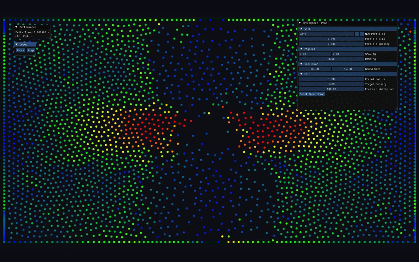
I built an interactive two-dimensional fluid simulation where the fluid is represented as particles instead of a fixed grid. Each particle stores its position, predicted position, velocity, density and mass. Their local interactions produce the global motion shown on screen.

The project runs on a custom engine that supplies the application loop, OpenGL rendering, an editor camera and ImGui controls. Particles are rendered as circles, the simulation boundary is drawn around them, and particle speed drives a heatmap color.

Why

The goal was to connect mathematical modeling with a tangible visual result. Fluid behavior is useful for that purpose because it requires turning abstract quantities—density, pressure, kernel radius and boundary response—into code that remains stable and responsive.

It was also an opportunity to study the trade-off between model fidelity and performance. A simulation that is accurate but cannot be explored interactively is less useful as an experimental tool.

How

Physics pipeline

Each fixed physics update follows an explicit pipeline: apply gravity, predict particle positions, rebuild the spatial lookup, compute density, compute pressure, integrate velocity and position, then resolve boundary collisions. The solver records timings for these stages and prints a performance breakdown every 60 frames.

The density estimator uses a Poly6 smoothing kernel. Pressure comes from the difference between the measured density and a configurable target density; the pressure force uses a Spiky gradient. The solver protects against zero densities and zero-distance neighbors before dividing or normalizing.

Neighborhood search

A naïve approach would compare every particle with every other particle. To avoid it, the solver creates a uniform grid using the current kernel radius as cell size. It stores (particleIndex, cellIndex) entries, sorts them by cell and records each cell’s starting offset. Each query then checks only the surrounding 3×3 cells and filters candidates by squared distance.

Time stepping and parallel work

The engine advances the model with a fixed timestep. Independent passes—gravity, predicted position, density, pressure, integration and collision response—use OpenMP parallel loops. Collisions clamp particles inside a configurable rectangular boundary and reverse velocity with a configurable damping factor.

grid.ForEachNearby(samplePoint, [&](int neighborIndex, float squaredDistance) {
    const float influence = SmoothingKernel(settings.KernelRadius, squaredDistance);
    density += particles[neighborIndex].mass * influence;
});

Results and learnings

The application exposes particle count, size, spacing, gravity, damping, bounds, kernel radius, target density and pressure multiplier through ImGui. Changing the kernel radius recomputes the kernel coefficients, and a reset action rebuilds the initial particle grid. This makes the simulation a compact environment for testing how local rules affect the whole system.

The central lesson was that performance decisions, such as the sorted spatial lookup, are part of the model design: they determine how much complexity can be explored in real time. Future iterations could add alternative boundary conditions, parameter presets and visual diagnostic layers for density and pressure.